This lesson has 3 virtues:

• manipulate bases of subspaces
• mix partial derivatives and vectors
• find an algorithm more efficient than the gradient method to solve $A \, {\bf x} = {\bf b}$

Conjugate gradient method

We have seen that it is possible to compute the optimal µ of the gradiant method to go directly to the minimum of the $J$ functional in along the line ${\bf x}^k \; + µ \, \nabla J({\bf x}^k)$ with µ varying from $- \infty$ at $+ \infty$ (see ma33).

We have also seen that if we have the optimal µ, then the next steepest slope, $\nabla J ({\bf x}^{k+1})$, will be orthogonal to the slope which defines the line on which we seek µ. So we have

$$\nabla J ({\bf x}^{k+1})^T \, . \, \nabla J ({\bf x}^k) = 0$$

This is good because it means that the next minimum, ${\bf x}^{k+2}$, will be the minimum of the space generated by $\nabla J ({\bf x}^{k+1})$ and $\nabla J ({\bf x}^k)$ (which is better than just being the minimum along a line).

Unfortunately nothing tells me that ${\bf x}^{k+3}$ will not be calculated along our first direction, $\nabla J({\bf x}^k)$. We have seen in the case of the gradient without searching for the optimal µ that we can oscillate between 2 values. That is not possible with the optimal µ but we can go around in circles on a few values.

Even if we don't go around in circles and we converge, is it likely that we are looking for again a minimum in a part of the $ℝ^n$ space that we have already explored.

An optimal search for the minimum of a convex function in a $ℝ^n$ space does not should not take more than $n$ iteration if we are still able to calculate the optimal µ in the chosen direction. To be convinced of this, it suffices to choose as directions the vectors of the basis of our space $ℝ^n$. Once we has found the minimum in all directions of the base, we have the global minimum. There is no longer any possible direction of search which would not be the linear combination of the vectors already used.

2D case

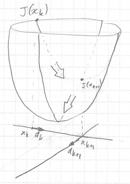
If we look for the point ${\bf x} = (x_1, x_2)$ which minimizes $J({\bf x})$ (convex) and that we know how to calculate the optimal µ of our gradient method, then we find the global minimum in 2 iterations at most. But id we take a too large µ which makes us pass above the minimum global, then at the next iteration the largest slope will be exactly the opposite of the one we just used and we will oscillate. On the drawing we can see that we find the global minimum in 2 iterations but we say to ourselves that it is a stroke of luck and besides is it really in 2 iterations since it is written ${\bf x}^k$? That's the limit of a drawing that wants to explain what is happening in $ℝ^n$ to humans accustomed to $ℝ^3$ (see this video on the 4th dimension outside classes).

Generate a base of $ℝ^n$

If we want to find our global minimum in $n$ maximum iteration, we must our directions is not redundant and therefore only the first $n$ directions generate $ℝ^n$ or form a basis of $ℝ^n$.

The new direction ${\bf d}^k$ must therefore be orthogonal to all directions preceding ones or that it makes it possible to find a base which generates a space of dimension $k+1$ (we start with ${\bf d}^0$).

Is it possible ?

The $A {\bf x} = {\bf b}$ case

In this case the functional to be minimized is

$$ J({\bf x}) = \frac{1}{2} \, {\bf x}^T \, A \, {\bf x} - {\bf b}\, . {\bf x} $$

and its gradient is $\nabla J({\bf x}) = A \; {\bf x} - {\bf b}$ if A is symmetrical.

We know that if we calculate ${\bf x}^k$ as before we only have orthogonality from two successive directions. It happens when µ is chosen to minimize $J$ along the direction line $\nabla J({\bf x}^k)$.

What happens if ${\bf x}^{k+1}$ minimizes $J$ in space ${\bf G_k}$ generated by all previous directions?

$$ J({\bf x}^{k+1}) = \min_{\bf v \in G_k} J({\bf x}^k + {\bf v}) $$ with ${\bf G_k} = span\{{\bf d}^0, {\bf d}^1,\dots, {\bf d}^k\} = \left\{ {\bf v} = \sum_{i=0}^{k} \alpha_i \, {\bf d}^i \quad \forall \alpha_i \in ℝ \right\}$.

Then all the partial derivatives with respect to the vectors of ${\bf G_k}$ are zero (just like $\partial J / \partial x$ and $\partial J / \partial y$ are zero at the minimum of J in the drawing above). Vector it is written like this:

$$ \nabla J({\bf x}^{k+1}) \, . \, {\bf w} = 0 \quad \forall {\bf w} \in {\bf G_k} $$

which is easily verified if ${\bf w}$ is one of the base vectors:

$$ \nabla J({\bf x}^{k+1}) \, . \, {\bf e}_i = \begin{bmatrix} \partial J / \partial x_{1} \\ \partial J / \partial x_{2} \\ \vdots \\ \partial J / \partial x_{i} \\ \vdots \\ \partial J / \partial x_{n} \\ \end{bmatrix} \, . \, \begin{bmatrix} 0 \\ 0 \\ \vdots \\ 1 \\ \vdots \\ 0 \\ \end{bmatrix} = \frac{\partial J}{\partial x_i}({\bf x}^{k+1}) $$

Note that saying the partial derivative of $J$ in a direction ${\bf w}$ of ${\bf G_k}$ is null, is equivalent to saying that $\nabla J({\bf x}^{k+1})$ is orthogonal to ${\bf w}$ (or null if $\nabla J({\bf x}^{k+1})$ the same dimension as ${\bf G_k}$).

Let's generate directions ${\bf d}^i$

So our iterative formula becomes:

$$ {\bf x}^{k+1} = {\bf x}^k - µ^k\, {\bf d}^k $$

To calculate the ${\bf d}^k$ we use the formula which tells us that the partial derivatives of $J$ with respect to a vector ${\bf w \in G_k}$ are null. And as the ${\bf d}^i$ directions generate the ${\bf G_k}$ space it is enough that the partial derivatives of $J$ with respect to all ${\bf d}^i$ are zero:

$$ \nabla J({\bf x}^{k+1}) \, . \, {\bf d}^i = 0 \quad \forall i \le k \qquad (1) $$

We perform the calculations

$$ \begin{align} (A\, {\bf x}^{k+1} - b) \, . \, {\bf d}^i &= 0 \quad \forall i \le k \\ (A\, ({\bf x}^{k} - µ^k \, {\bf d}^k) - b) \, . \, {\bf d}^i &= 0 \quad \forall i \le k \\ (A\, {\bf x}^{k} - b) \, . \, {\bf d}^i - µ^k \, A \, {\bf d}^k \, . \, {\bf d}^i &= 0 \quad \forall i \le k \\ \nabla J({\bf x}^{k}) \, . \, {\bf d}^i - µ^k \, A \, {\bf d}^k \, . \, {\bf d}^i &= 0 \quad \forall i \le k \\ \end{align} $$

If $i < k$ then the first term is zero which gives

$$ A \, {\bf d}^k \, . \, {\bf d}^i = 0 \quad \forall i < k \qquad (2) $$

As A is symmetric, we also have $A \, {\bf d}^i \, . \, {\bf d}^k = 0 \quad \forall i < k\quad$ ($\sum_{m=1}^N \sum_{n=1}^N a_{m,n}\, d^i_n\, d^k_m = \sum_{n=1}^N \sum_{m=1}^N a_{n,m}\, d^k_m\, d^i_n$).

So we have conditions to build the new direction ${\bf d}^k$.

We assume that the new direction is the gradient + a correction which is a linear combination of the previous directions: $$ {\bf d}^k = \nabla J({\bf x}^k) + \sum_{j=0}^{k-1} β_j {\bf d}^j $$ then equation (2) becomes $$ A \, \left( \nabla J({\bf x}^k) + \sum_{j=0}^{k-1} β_j {\bf d}^j \right) . {\bf d}^i = 0 \quad \forall i < k $$ The sum will reveal $A\, {\bf d}^j {\bf d}^i$ which are all null according to (2) and its symmetric version except $A\, {\bf d}^i {\bf d}^i$. So

$$ β_i = - \frac{A\, \nabla J({\bf x}^k) \, . \, {\bf d}^i}{A\, {\bf d}^i \, . \, {\bf d}^i} $$

and so $$ {\bf d}^k = \nabla J({\bf x}^k) - \sum_{i=0}^{k-1} \frac{A\, \nabla J({\bf x}^k) \, . \, {\bf d}^i} {A\, {\bf d}^i \, . \, {\bf d}^i} \; {\bf d}^i $$

Calculation of $μ^k$

We have seen that $\nabla J({\bf x}^{k+1}) \, . \, {\bf d}^i = 0$ gives

$$ \nabla J({\bf x}^{k}) \, . \, {\bf d}^i - µ^k \, A \, {\bf d}^k \, . \, {\bf d}^i = 0 \quad \forall i \le k $$

so also for $i = k$ which allows to calculate $μ^k$:

$$ µ^k = \frac{\nabla J({\bf x}^{k}) \, . \, {\bf d}^k} {A \, {\bf d}^k \, . \, {\bf d}^k} = \frac{(A \, {\bf x}^{k} - b) \, . \, {\bf d}^k} {A \, {\bf d}^k \, . \, {\bf d}^k} \\ \, $$

We therefore have the method to calculate ${\bf d}^k$ and $µ^k$ which makes it possible to find ${\bf x}^{k+1}$ from ${\bf x}^k$.

Property

$$ \nabla J({\bf x}^{k+1}) \perp \nabla J({\bf x}^i) \quad \forall i \le k $$

Exercise Prove this property by induction starting from (0), knowing that the first direction is ${\bf d}^0 = \nabla J({\bf x}^0)$.

This property shows that the set of gradients of $J$ at points ${\bf x}^i$ form a basis of space $\bf G_k$. So we are sure that our algorithm converges in $n$ iterations at most.

2nd attempt

The method found is good because it shows that we can optimize the gradient descent but the calculation of ${\bf d}^k$ is way too heavy. So we're going to start all over again to find another more efficient way.

Let's work in the base of $\nabla J({\bf x}^i)$

We start from equation (0) which allows us to show that the $\nabla J({\bf x}^i), i \le k$ form a basis of the subspace $\bf G_k$. Also any vector is expressed in this basis and therefore

$$ {\bf x}^{k+1} = {\bf x}^k + μ^k \, {\bf d}^k \quad \textrm{avec} \quad {\bf d}^k = - \nabla J({\bf x}^k) + \sum_{i=0}^{k-1} γ^i \, \nabla J({\bf x}^i) $$

Note that these ${\bf d}^i, i \le k$ also form a basis of $\bf G_k$.

Equation (2) tells us that $A \, {\bf d}^k \, . \, {\bf d}^i = 0 \quad \forall i < k$, therefore

$$ \begin{align} < A \, {\bf d}^k, {\bf x}^{j+1} - {\bf x}^j > &= 0 \quad \forall j < k \\ < {\bf d}^k, A \, ({\bf x}^{j+1} - {\bf x}^j) > &= 0 \quad \textrm{since A is symetrical} \\ < {\bf d}^k, A \, {\bf x}^{j+1} - {\bf b} - A {\bf x}^j + {\bf b} > &= 0 \\ < {\bf d}^k, \nabla J({\bf x}^{j+1}) - \nabla J({\bf x}^j) > &= 0 \\ < - \nabla J({\bf x}^k) + \sum_{i=0}^{k-1} γ^i \, \nabla J({\bf x}^i) , \nabla J({\bf x}^{j+1}) - \nabla J({\bf x}^j) > &= 0 \quad (3) \\ \end{align} $$

If j = k-1 then $$ \begin{align} < - \nabla J({\bf x}^k), \nabla J({\bf x}^k) > + \, γ^{k-1} < \nabla J({\bf x}^{k-1}), -\nabla J({\bf x}^{k-1}) > &= 0 \\ γ^{k-1} = -\frac{< \nabla J({\bf x}^{k}), \nabla J({\bf x}^{k}) >} {< \nabla J({\bf x}^{k-1}), \nabla J({\bf x}^{k-1}) >} \end{align} $$

If j = k-2 then $$ \begin{align} γ^{k-1} \, < \nabla J({\bf x}^{k-1}), \nabla J({\bf x}^{k-1}) > + \, γ^{k-2} < \nabla J({\bf x}^{k-2}), -\nabla J({\bf x}^{k-2}) > &= 0 \\ γ^{k-2} = γ^{k-1} \frac{< \nabla J({\bf x}^{k-1}), \nabla J({\bf x}^{k-1}) >} {< \nabla J({\bf x}^{k-2}), \nabla J({\bf x}^{k-2}) >} = \frac{< \nabla J({\bf x}^{k}), \nabla J({\bf x}^{k}) >} {< \nabla J({\bf x}^{k-2}), \nabla J({\bf x}^{k-2}) >} \end{align} $$ and continuing the calculations, we have $\forall j < k-1$ $$ γ^j = \frac{< \nabla J({\bf x}^{k}), \nabla J({\bf x}^{k}) >} {< \nabla J({\bf x}^{j}), \nabla J({\bf x}^{j}) >} $$

The general formula of ${\bf d}^k$ is therefore $$ \begin{align} {\bf d}^k &= -\nabla J({\bf x}^k) - \frac{< \nabla J({\bf x}^{k}), \nabla J({\bf x}^{k}) >} {< \nabla J({\bf x}^{k-1}), \nabla J({\bf x}^{k-1}) >} \, \nabla J({\bf x}^{k-1}) + \sum_{i=0}^{k-2} \frac{< \nabla J({\bf x}^{k}), \nabla J({\bf x}^{k}) >} {< \nabla J({\bf x}^{i}), \nabla J({\bf x}^{i}) >} \, \nabla J({\bf x}^i) \\ &= -\nabla J({\bf x}^k) + β \left( -\nabla J({\bf x}^{k-1}) + \sum_{i=0}^{k-2} \frac{< \nabla J({\bf x}^{k-1}), \nabla J({\bf x}^{k-1}) >} {< \nabla J({\bf x}^{i}), \nabla J({\bf x}^{i}) >} \, \nabla J({\bf x}^i) \right) \\ &= -\nabla J({\bf x}^k) + β \, {\bf d}^{k-1} \quad \textrm{with} \quad β = \frac{< \nabla J({\bf x}^{k}), \nabla J({\bf x}^{k}) >} {< \nabla J({\bf x}^{k-1}), \nabla J({\bf x}^{k-1}) >} \end{align} $$

We have therefore succeeded in expressing the new direction only as a function of the current gradient and the previous direction.

New calculation of μ

The previous calculation of μ remains valid since this calculation does not depend on the way of expressing ${\bf d}^k$.

$$ µ^k = -\frac{\nabla J({\bf x}^{k}) \, . \, {\bf d}^k} {A \, {\bf d}^k \, . \, {\bf d}^k} \, $$

With our choice of ${\bf d}^k$ this gives

$$ µ^k = -\frac{<\nabla J({\bf x}^{k}), - \nabla J({\bf x}^{k}) + β \, {\bf d}^{k-1}>} {<A \, {\bf d}^k, {\bf d}^k>} = \frac{<\nabla J({\bf x}^{k}), \nabla J({\bf x}^{k})>} {<A \, {\bf d}^k, {\bf d}^k>} $$ since ${\bf d}^{k-1} \perp \nabla J({\bf x}^{k})$.