The gradient method to solve A x = b

The goal of this lab is to let you move forward on your own. Look at previous course and program the gradient method to solve the $A {\bf x} = {\bf b}$ matrix system with A symmetric and diagonally dominant ($a_{ii} > \sum_{k \ne i} |a_{ik}|$).

• Start in 2D with a 2x2 matrix, check that the result is good and plot the convergence curve
• Switch to nxn (we will show that it works with a 9x9 matrix)

It may be interesting to normalize the matrix A to prevent the calculations from exploding.

def solve_with_gradiant(A, b):
    mu = 0.01

import numpy as np
A = np.random.randint(10, size=(2,2))
A = A + A.T
A += np.diag(A.sum(axis=1))
A

array([[49, 13],
       [13, 13]])

b = A.sum(axis=1)
b

array([62, 26])

solve_with_gradiant(A,b)

Introduce inertia

Introduce inertia into the gradient method. What do we notice?

Optimal value of µ

Note that two successive slope directions are orthogonal if the next point is the minimum in given direction ($\nabla J ({\bf x}^k$)).

$$\nabla J ({\bf x}^{k+1})^T \; \nabla J ({\bf x}^k) = 0$$

Demonstration

We want to adjust µ to arrive at the minimum of J when we advance in the direction $- \nabla J({\bf x}^{k})$. This means that the partial derivative of $J({\bf x}^{k+1})$ with respect to µ must be equal to 0 or by making µ appear in the equation: $$ \frac{\partial J ({\bf x}^k - µ \; \nabla J ({\bf x}^k))}{\partial µ} = 0 $$ By expanding we have $$ \begin{align} \frac{\partial J ({\bf x}^{k+1})}{\partial {\bf x}^{k+1}} \; \frac{\partial {\bf x}^{k+1}}{\partial µ} & = 0 \\ J'({\bf x}^{k+1}) \, . \, (- \nabla J ({\bf x}^k)) & = 0 \\ (A\, {\bf x}^{k+1} - b) \, . \, \nabla J ({\bf x}^k) & = 0 \quad \textrm{since A is symetric}\\ \nabla J ({\bf x}^{k+1}) \, . \, \nabla J ({\bf x}^k) & = 0 \quad \textrm{QED} \end{align} $$

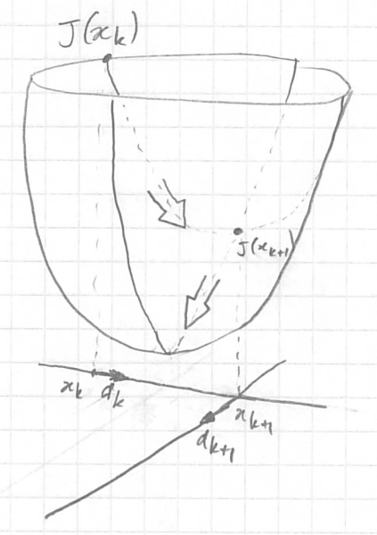
Using this property, evaluate the optimal value of µ to reach the minimum in the direction of $\nabla J ({\bf x}^k)$.

Write the gradient method with the calculation of the optimal µ at each iteration to solve $A {\bf x} = {\bf b}$.