import numpy as np
import numpy.linalg as lin

np.set_printoptions(precision=3, linewidth=150, suppress=True)
np.random.seed(123)
Numerical simulation
If the price of bananas is important, the sector with the greatest system resolution needs matrices is numerical simulation. This includes this
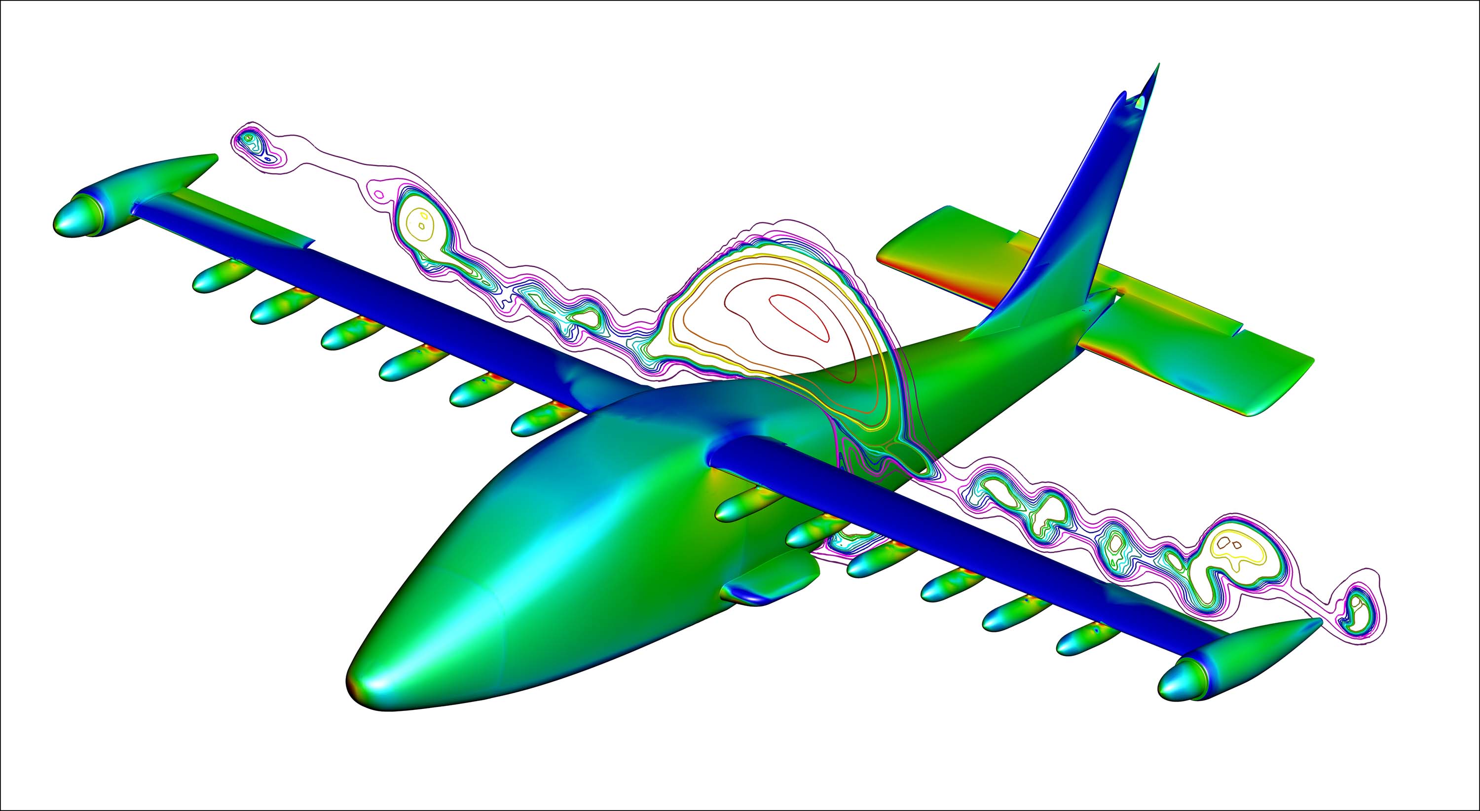
and everything that is digitally simulated, namely everything related to transport, energy, construction, everything what we manufacture, which is expensive and which must have a very specific physical behavior. But that's not all, understanding our environment (weather, global warming, chemistry, etc.) also means solving matrix systems as well as other areas. However, there are numerical simulation methods that do not go through matrix systems.
To make the image above, we transform physical equations like Navier-Stokes into a matrix system where the unknowns are defined at each point of a mesh to be defined. In our case the unknown is the pressure and the mesh is the interior of a imaginary box that includes the plane and the air that circulates around it.
If the box is a cube with 1000 points in each direction, we have 1 billion points in the box (minus what is inside the plane but let's stay on 1 billion). Then the matrix has 1 quadrillion elements (one billion squared).
$$ \begin{bmatrix} a_{11} \; a_{12} \ldots a_{1,10^9} \\ a_{21} \; a_{22} \ldots a_{2,10^9} \\ \vdots \\ a_{10^9,1} a_{n2} \ldots a_{10^9,10^9} \\ \end{bmatrix} \; \begin{bmatrix} p_{1} \\ p_{2} \\ \vdots \\ p_{10^9} \\ \end{bmatrix} = \begin{bmatrix} f_{1} \\ f_{2} \\ \vdots \\ f_{10^9} \\ \end{bmatrix} $$
Inverting a matrix is done in $O(n³)$ operations or $O(10^{27})$ in our case.
If you have the most powerful computer in the world in 2024 you can do 1 Eflops or $10^{18}$ operations per second. Also you will need $10^{9}$ seconds or a little over 30 years. It's too much.
Inverting a matrix or solving by a direct method is not the right solution to solve a large matrix system.
Exercise 12.1
For such a simulation it is also necessary to calculate the speed of the air in each of the 1 billion points of our grid. A speed is 3 variables that must be added to the pressure. How long does it take to reverse the matrix which also integrates the speed of the air?
# ceci est une calculatrice, vous pouvez donc écrire la réponse ici
It is a good idea to estimate the time of a large calculation before launching it.
Besides, with such long times, he should not stay with orders of magnitude but specify with the exact formula. So with Choleski it's $n^3/3$ operations therefore it runs 3 times faster, but it is still too much.
Iterative Methods
Iterative methods are methods that approach the desired solution step by step. They allow to find an approximation of ${\bf x}$, the solution of $A\, {\bf x} = b$.
In general we stops the calculation when we estimate that we are at a chosen distance from the solution (which we call the error) rather than waiting to be at the exact solution. Anyway the exact solution on a computer which is limited in number of decimal places can be unattainable. So we will never seek to have an error smaller than our maximum precision.
The fundamental idea of the iterative algorithm is to have a formula like $\; {\bf x}^{t+1} = B \, {\bf x}^t + {\bf c}\;$ or in Python:
x = np.random(size = c.size)
while np.square(x - old_x) > threshold:
    old_x = x
    x = B @ x + c
The magic is if x converges. In this case we have reached a fixed point i.e. that ${\bf x}^{t+1} = {\bf x}^t$ and so
$${\bf x}^t = B \, {\bf x}^t + {\bf c} \quad \textrm{c.a.d.} \quad (Id -B) \, {\bf x}^t = {\bf c}$$
We find our $A \; {\bf x} = {\bf b}$ that being in practice we do not cut A into Id and B because ca does not converge (except particular cases). Let's see how the Jacobi method does it.
Jacobi method
The Jacobi method cuts the matrix A into M and N with
M the diagonal matrix that includes the elements of the diagonal of A N = M - A (so 0 on the diagonal and the opposite of the elements of A elsewhere)
So the system to solve is $\; (M - N) \, {\bf x} = {\bf b}$.
The iterative formula is therefore for iteration k+1 expressed as a function of iteration k:
$$ M \; {\bf x}^{k+1} = N\; {\bf x}^k + {\bf b} $$
and since M is a diagonal matrix, we have:
$$ \begin{array}{l} a_{11} x_1^{k+1} = \qquad -a_{12} \, x_2^k - a_{13} \, x_3^k \ldots - a_{1n} \, x_n^k + b_1 \\ a_{22} x_2^{k+1} = -a_{21} \, x_1^k \qquad - a_{23} \, x_3^k \ldots - a_{2n} \, x_n^k + b_2 \\ a_{33} x_3^{k+1} = -a_{31} \, x_1^k - a_{32} \, x_3^k \qquad \ldots - a_{3n} \, x_n^k + b_3 \\ \vdots \\ a_{nn} x_n^{k+1} = -a_{n1} \, x_1^k - a_{n2} \, x_3^k \ldots - a_{n-1,n-1} \, x_{n-1}^k \qquad + b_n \\ \end{array} $$
We see in watermark $A \; {\bf x} = {\bf b}$.
To calculate $x_1^{k+1}$ it is necessary to divide the right term of the first line by $a_{11}$ it is thus necessary that $a_{11} \ne 0$.
To calculate the following terms $x_i^{k+1}$ it is also necessary that $a_{ii}$ be non-zero so it A must not have zero on its diagonal.
This can be found in the following writing, which takes up the initial formula: $ {\bf x}^{k+1} = M^{-1} \;(N\; {\bf x}^k + {\bf b})$
We see that in order to be effective, M must be easily invertible, otherwise we might as well invert A directly. Here it is indeed the case since M is diagonal.
Let's program Jacobi
A = np.random.randint(10, size=(4,4))
b = A.sum(axis=1)                     # ainsi la solution est [1,1,1,1]
print('A:\n', A, "\nb:\n", b, "\n")

M = np.diag(A)        # attention, c'est un vecteur
N = np.diag(M) - A    # np.diag d'une matrice donne un vecteur, np.diag d'un vecteur donne une matrice
print(f"M:\n {np.diag(M)}\nN:\n {N}\n")

x = np.random.random(4)
for i in range(20):
    print(f"x_{i} = {x}")
    x = (N @ x + b) / M
A:
 [[2 2 6 1]
 [3 9 6 1]
 [0 1 9 0]
 [0 9 3 4]]
b:
 [11 19 10 16]

M:
 [[2 0 0 0]
 [0 9 0 0]
 [0 0 9 0]
 [0 0 0 4]]
N:
 [[ 0 -2 -6 -1]
 [-3  0 -6 -1]
 [ 0 -1  0  0]
 [ 0 -9 -3  0]]

x_0 = [0.398 0.738 0.182 0.175]
x_1 = [4.127 1.837 1.029 2.203]
x_2 = [-0.526 -0.195  0.907 -0.906]
x_3 = [3.427 1.782 1.133 3.759]
x_4 = [-1.56  -0.204  0.913 -0.86 ]
x_5 = [3.395 2.118 1.134 3.775]
x_6 = [-1.907 -0.196  0.876 -1.616]
x_7 = [3.877 2.342 1.133 3.784]
x_8 = [-2.133 -0.357  0.851 -2.12 ]
x_9 = [4.364 2.49  1.151 4.165]
x_10 = [-2.525 -0.574  0.834 -2.467]
x_11 = [4.804 2.671 1.175 4.665]
x_12 = [-3.027 -0.792  0.814 -2.89 ]
x_13 = [5.293 2.898 1.199 5.17 ]
x_14 = [-3.581 -1.027  0.789 -3.421]
x_15 = [5.87  3.159 1.225 5.719]
x_16 = [-4.194 -1.298  0.76  -4.026]
x_17 = [6.531 3.45  1.255 6.35 ]
x_18 = [-4.891 -1.608  0.728 -4.704]
x_19 = [7.277 3.779 1.29  7.073]
It doesn't really converge... (if you rerun and see NaN it means there is a zero on the diagonal)
2nd try:
A = np.random.randint(10, size=(4,4))
A = A + np.diag(A.sum(axis=0))
b = A.sum(axis=1)                     # ainsi la solution est [1,1,1,1]
print('A:\n', A, "\nb:\n", b, "\n")


M = np.diag(A)        # attention, c'est un vecteur
N = np.diag(M) - A    # np.diag d'une matrice donne un vecteur, np.diag d'un vecteur donne une matrice
print(f"M:\n {np.diag(M)}\nN:\n {N}\n")

x = np.random.random(4)
for i in range(20):
    print(f"x_{i} = {x}")
    x = (N @ x + b) / M
A:
 [[24  2  4  8]
 [ 0 24  9  3]
 [ 4  6 16  5]
 [ 6  2  1 32]]
b:
 [38 36 31 41]

M:
 [[24  0  0  0]
 [ 0 24  0  0]
 [ 0  0 16  0]
 [ 0  0  0 32]]
N:
 [[ 0 -2 -4 -8]
 [ 0  0 -9 -3]
 [-4 -6  0 -5]
 [-6 -2 -1  0]]

x_0 = [0.766 0.777 0.028 0.174]
x_1 = [1.456 1.468 1.4   1.088]
x_2 = [0.865 0.839 0.683 0.873]
x_3 = [1.109 1.135 1.134 1.045]
x_4 = [0.951 0.944 0.908 0.967]
x_5 = [1.031 1.039 1.043 1.015]
x_6 = [0.984 0.982 0.973 0.99 ]
x_7 = [1.009 1.011 1.014 1.005]
x_8 = [0.995 0.994 0.992 0.997]
x_9 = [1.003 1.003 1.004 1.002]
x_10 = [0.998 0.998 0.998 0.999]
x_11 = [1.001 1.001 1.001 1.   ]
x_12 = [1.    0.999 0.999 1.   ]
x_13 = [1. 1. 1. 1.]
x_14 = [1. 1. 1. 1.]
x_15 = [1. 1. 1. 1.]
x_16 = [1. 1. 1. 1.]
x_17 = [1. 1. 1. 1.]
x_18 = [1. 1. 1. 1.]
x_19 = [1. 1. 1. 1.]
Magic!
Why does the 2nd case work?
For an iterative method of the ${\bf x} = B\; {\bf x} + {\bf c}$ type to converge, it is necessary to choose
- $\rho(B) < 1\quad$ with $\rho$ the spectral radius (which is the largest eigenvalue in absolute value)
- $||B|| < 1\quad$ with a matrix norm is subordinate to a vector norm.
Case of the Jacobi method
For the Jacobi matrix B, these conditions are met if A is at dominant diagonal, namely that each diagonal element is greater in modulus than the sum of all other modulus elements in its row or column ($|a_{i,i}| \ge \sum_{j \ne i} |a_{i,j}|$).
Jacobi also converges if A is symmetric, real and positive definite (i.e. $\forall {\bf x}, \; {\bf x}^T \, A \, {\bf x} > 0$).
Calculation time
If we converge in 10 iterations then 10 matrix multiplications, 10 vector additions and 10 vector divisions are used, i.e. 180 operations to be compared to the $4^3 / 3 = 22$ operations of a direct method. Damn !
Some reasons why we lose are
- Matrix A is too small, iterative methods are interesting for large matrices
- Jacobi's method is not the best (but it is very easily parallelizable)
- The spectral radius of the matrix is too large. The greater the spectral radius smaller and the faster we converge.