Principal component analysis (PCA)

import numpy as np
import matplotlib.pyplot as plt
import numpy.linalg as lin

%matplotlib inline
%config InlineBackend.figure_format = 'retina'

np.set_printoptions(precision=3, linewidth=150, suppress=True)
plt.style.use(['seaborn-whitegrid','data/cours.mplstyle'])

import matplotlib

def arrow2D(a,b, color='k', **kargs):
    astyle = matplotlib.patches.ArrowStyle("simple", head_length=.8, head_width=.8, tail_width=.1)
    plt.plot([a[0],b[0]], [a[1],b[1]] ,visible = False) # to define the visible windows
    plt.annotate("", xytext=a, xy=b, 
                 arrowprops=dict(arrowstyle=astyle, shrinkA=0, shrinkB=0, aa=True, color=color, **kargs))

A cloud of dots

When we have a cloud of points we can study its shape by a principal component analysis (PCA). This comes back to seek the eigenvectors of the covariance matrix (or correlation which is the covariance matrix normalized by the standard deviations). These eigenvectors describe the point cloud to us.

To check it, let's make a scatter plot with a strong correlation between $x$ and $y$:

$$ y = 0.2 \, x + 1.45 + U(-1,1) \quad \textrm{avec U la loi uniforme qui simule du bruit.}$$

This linear relation between $x$ and $y$ allows us to know that we have:

a slope of 0.2 a vertical offset of 1.45 in x=0

The goal is to see if, with only the scatter plot, we can find the correlation between $x$ and $y$ despite the noise.

$$ y = α x + β$$

N = 50
x = 10 * np.random.rand(N) - 5
nuage = np.array([x, 0.2 * x + 1.45 + (2 * np.random.rand(N) - 1)])

plt.plot(nuage[0], nuage[1], 'x')
plt.title('Un nuage de points')
plt.axis('equal');

Graphically, we are looking for the line that minimizes the distance between the points and their projection on the line.

We can also construct the covariance matrix (see below) and see that the slope of the first eigenvector is equal to this coefficient 0.2 which connects x to y.

Then the average of the point cloud in a point of the line that we are looking for, which means that with the direction vector that is the first eigenvector, we have our line.

cov = np.cov(nuage.copy())
cov

array([[9.107, 1.925],
       [1.925, 0.764]])

Let us take this opportunity to recall that if a matrix is ​​symmetric then

• its eigenvalues are real
• its eigenvectors are orthogonal

val, vec = lin.eig(cov)
val = val.astype('float')  # on convertit puisqu'on sait que ce sont des réels
print("Valeurs propres de la matrice de covariance :", val,"\n")
print("Vecteurs propres de la matrice de covariance :\n", vec)

Valeurs propres de la matrice de covariance : [9.53  0.341] 

Vecteurs propres de la matrice de covariance :
 [[ 0.977 -0.215]
 [ 0.215  0.977]]

/tmp/ipykernel_26870/3419464211.py:2: ComplexWarning: Casting complex values to real discards the imaginary part
  val = val.astype('float')  # on convertit puisqu'on sait que ce sont des réels

plt.plot(nuage[0], nuage[1], 'x')
arrow2D((0,0), val[0] * vec[:,0], 'r')  # vecteur propre multiplié par sa valeur propre
arrow2D((0,0), val[1] * vec[:,1], 'g')
plt.title('Un nuage de points et les vecteurs propres de sa matrice de covariance')
plt.axis('equal');

Let's check that the slope of the first eigenvector is close to 0.2:

pente = vec[1,0] / vec[0,0]  
print("La pente est de", pente, '\n')
moyenne = nuage.mean(axis=1)
print("Le points moyen du nuage est", moyenne)

La pente est de 0.21963615318288862 

Le points moyen du nuage est [-0.152  1.327]

eq_droite = lambda x: pente * (x - moyenne[0]) + moyenne[1]

print("Le décalage verticale est de ", eq_droite(0))

plt.plot(nuage[0], nuage[1], 'x')
plt.plot([nuage[0].min(), nuage[0].max()], [eq_droite(nuage[0].min()), eq_droite(nuage[0].max())]) 
plt.title("Un nuage de points et sa droite d'approximation")
plt.axis('equal');

Le décalage verticale est de  1.360408912029785

print(f'On a donc α = {pente:.3f} et β = {eq_droite(0):.3f} sachant que le nuage a été généré avec 0.2 et 1.45')

On a donc α = 0.220 et β = 1.360 sachant que le nuage a été généré avec 0.2 et 1.45

Covariance matrix

The covariance between two datasets x and y indicates how closely they are related (i.e. if the i-th value of y can be deduced from the i-th value of x or not). If their covariance is large in absolute value then they are strongly related, if it is close to 0, they are either independent is linked by a more complicated relationship than a simple linear relationship.

Covariance measures the linear relationship between 2 variables (see this video for a quick and complete presentation of covariance and its properties).

$$ \textrm{cov}(\textbf{x},\textbf{y}) = \frac{1}{N} \sum_{i=1}^N (x_i - \overline{\textbf{x}}) (y_i - \overline{\textbf{y}}) $$

with $N$ the number of points of the cloud, $\overline{\textbf{x}}$ and $\overline{\textbf{y}}$ the averages of $\textbf{x}$ and $\textbf{y}$.

If we place the origin of the axes at the mean $(\overline{\textbf{x}},\overline{\textbf{y}})$ then the formula indicates that to have correlation there must be more points in 2 diagonally opposite quadrans.

If, conversely, we draw random points, so no relationship between x and y, then we will have points distributed evenly around the mean, so a zero covariance. Finally if all the values ​​of $\textbf{y}$ have the same value, then they do not depend on x and $y_i - \overline{\textbf{y}} = 0 \; \forall i$ so the covariance is zero.

plt.plot(nuage[0], nuage[1], 'x')
plt.plot([moyenne[0], moyenne[0]], [nuage[1].min(), nuage[1].max()],'k')
plt.plot([nuage[0].min(), nuage[0].max()], [moyenne[1], moyenne[1]],'k')
plt.title('La covariance indique une direction privilégiée et donc plus de points dans les quadrans traversés')
plt.axis('equal');

Here we can clearly see that the vast majority of points are in 2 opposite quadrans, of which our 2 variables are linked.

The covariance matrix expresses all the possible covariances between the variables. In our case where the cloud has 2 dimensions, we have:

$$ \textrm{Cov(nuage 2D)} = \begin{bmatrix} \textrm{cov}(\textbf{x},\textbf{x}) & \textrm{cov}(\textbf{x},\textbf{y}) \\ \textrm{cov}(\textbf{y},\textbf{x}) & \textrm{cov}(\textbf{y},\textbf{y}) \\ \end{bmatrix} $$

cov = lambda x,y : np.dot((x - x.mean()), (y - y.mean())) / len(x)

Cov = lambda x,y : np.array([[cov(x,x), cov(x,y)], [cov(y,x), cov(y,y)]])

Cov(nuage[0], nuage[1]) # par défaut Numpy divise par (N-1), avec bias=True il divise par N et donne ce résultat

array([[8.925, 1.887],
       [1.887, 0.749]])

This result shows that x is very linked with itself, which is obvious. On the other hand, it seems that there is less connected with himself. In fact the variations of y are smaller (between 0 and 3 while x varies between -5 and 5) which explains this smaller value. The fact that cov(x,y) is greater than cov(y,y) is already a indicator that x and y are related.

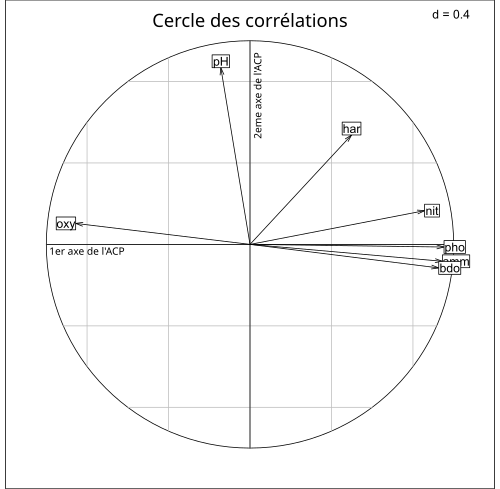
The calculation of the eigenvalues ​​and vectors of the covariance matrix is ​​even more interesting with a large dimension because it highlights which are the most important. Thus the example of the article from Wikipedia on 'principal component analysis on the pollution of the Doubs water shows that the first clean vector is that of known pollutants: nitrates (nit), phosphates (pho), ammonia (amm) and the second is that of PH. Note the anti-correlation between oxygen content and pollutants.

To fully understand this figure and see a use case, I invite you to watch this example of PCA with Excel.